
Rを用いて生存分析を行う際に, Kaplan-Meier curve に打ち切りのマークを入れたり,number at risk (at risk table)を併記する方法はすぐに見つかるが(Drawing survival curves in R, ggkm, Survival plots have never been so informative),competing riskのplotの場合はあまり情報がない.prodlimを使えば簡単なので,まとめておく.
なお, competing risk については以下を参照.
- Competing risk analysis using R: an easy guide for clinicians
- Regression modeling of competing risk using R: an in depth guide for clinicians
- Competing risk analysisのデモ
- A not so short review on survival analysis in R
Table of Contents
Prepare dataset “Melanoma” from “riskRegression” package
library(riskRegression)
data(Melanoma)
head(Melanoma)
summary(Melanoma)
  time status                    event invasion ici      epicel       ulcer
1   10      2       death.other.causes  level.1   2     present     present
2   30      2       death.other.causes  level.0   0 not present not present
3   35      0                 censored  level.1   2 not present not present
4   99      2       death.other.causes  level.0   2 not present not present
5  185      1 death.malignant.melanoma  level.2   2     present     present
6  204      1 death.malignant.melanoma  level.2   2 not present     present
  thick    sex age   logthick
1  6.76   Male  76  1.9110229
2  0.65   Male  56 -0.4307829
3  1.34   Male  41  0.2926696
4  2.90 Female  71  1.0647107
5 12.08   Male  52  2.4915512
6  4.84   Male  28  1.5769147
      time          status                            event        invasion
 Min.   :  10   Min.   :0.0000   censored                :134   level.0:99
 1st Qu.:1525   1st Qu.:0.0000   death.malignant.melanoma: 57   level.1:77
 Median :2005   Median :0.0000   death.other.causes      : 14   level.2:29
 Mean   :2153   Mean   :0.4146
 3rd Qu.:3042   3rd Qu.:1.0000
 Max.   :5565   Max.   :2.0000
 ici             epicel            ulcer         thick           sex
 0: 17   not present:116   not present:115   Min.   : 0.10   Female:126
 1: 59   present    : 89   present    : 90   1st Qu.: 0.97   Male  : 79
 2:107                                       Median : 1.94
 3: 22                                       Mean   : 2.92
                                             3rd Qu.: 3.56
                                             Max.   :17.42
      age           logthick
 Min.   : 4.00   Min.   :-2.30259
 1st Qu.:42.00   1st Qu.:-0.03046
 Median :54.00   Median : 0.66269
 Mean   :52.46   Mean   : 0.61817
 3rd Qu.:65.00   3rd Qu.: 1.26976
 Max.   :95.00   Max.   : 2.85762
Competing risk analysis with cuminc of “cmprsk” package
- cuminc is used to investigate whether a statistically significant difference is present between the groups (see “Tests:” below).
library(cmprsk)
Results_cmprsk <- with(Melanoma, cuminc(time, event, group = sex, cencode = "censored"))
Results_cmprsk
Tests:
                              stat        pv df
death.malignant.melanoma 5.8140209 0.0158989  1
death.other.causes       0.8543656 0.3553203  1
Estimates and Variances:
$est
                                      1000       2000       3000       4000
Female death.malignant.melanoma 0.08730159 0.18077594 0.23565169 0.28424490
Male death.malignant.melanoma   0.19237175 0.31009828 0.42453587 0.42453587
Female death.other.causes       0.03174603 0.03983516 0.05220642 0.08538385
Male death.other.causes         0.03814124 0.06693942 0.06693942 0.13474271
                                      5000
Female death.malignant.melanoma 0.28424490
Male death.malignant.melanoma           NA
Female death.other.causes       0.08538385
Male death.other.causes                 NA

$var
                                        1000         2000         3000
Female death.malignant.melanoma 0.0006378135 0.0012450462 0.0018102025
Male death.malignant.melanoma   0.0020223293 0.0028196248 0.0042695603
Female death.other.causes       0.0002459647 0.0003073878 0.0004529114
Male death.other.causes         0.0004727379 0.0008614343 0.0008614343
                                       4000        5000
Female death.malignant.melanoma 0.002755577 0.002755577
Male death.malignant.melanoma   0.004269560          NA
Female death.other.causes       0.001528480 0.001528480
Male death.other.causes         0.002950698          NA
Competing risk analysis with prodlim
Days
CompRskAnalysis <- prodlim(Hist(time, status, cens.code=0) ~ sex, data = Melanoma)
summary(CompRskAnalysis)
----------> Cause:  1

sex=Female :
  time n.risk n.event n.lost cuminc se.cuminc  lower upper
1   10    126       0      0  0.000    0.0000 0.0000 0.000
2 1513    104       0      0  0.127    0.0297 0.0688 0.185
3 2006     67       0      0  0.181    0.0351 0.1120 0.250
4 3042     34       0      0  0.236    0.0423 0.1528 0.318
5 5565      1       0      1  0.284    0.0519 0.1826 0.386

sex=Male :
  time n.risk n.event n.lost cuminc se.cuminc lower upper
1   10     79       0      0  0.000    0.0000 0.000 0.000
2 1513     51       0      0  0.270    0.0503 0.171 0.368
3 2006     35       0      0  0.310    0.0527 0.207 0.413
4 3042     18       0      0  0.425    0.0644 0.298 0.551
5 5565      0       0      0     NA        NA    NA    NA


----------> Cause:  2

sex=Female :
  time n.risk n.event n.lost cuminc se.cuminc   lower  upper
1   10    126       0      0 0.0000    0.0000 0.00000 0.0000
2 1513    104       0      0 0.0317    0.0156 0.00113 0.0624
3 2006     67       0      0 0.0398    0.0175 0.00562 0.0741
4 3042     34       0      0 0.0522    0.0212 0.01073 0.0937
5 5565      1       0      1 0.0854    0.0383 0.01027 0.1605

sex=Male :
  time n.risk n.event n.lost cuminc se.cuminc   lower  upper
1   10     79       1      0 0.0127    0.0126 0.00000 0.0373
2 1513     51       0      0 0.0510    0.0248 0.00230 0.0996
3 2006     35       0      0 0.0669    0.0291 0.00992 0.1240
4 3042     18       0      0 0.0669    0.0291 0.00992 0.1240
5 5565      0       0      0     NA        NA      NA     NA
Years
CompRskAnalysis2 <- prodlim(Hist(time/365.25, event, cens.code="censored") ~ sex, data = Melanoma)
summary(CompRskAnalysis2)
----------> Cause:  death.malignant.melanoma

sex=Female :
     time n.risk n.event n.lost cuminc se.cuminc  lower upper
1  0.0274    126       0      0  0.000    0.0000 0.0000 0.000
2  4.1424    104       0      0  0.127    0.0297 0.0688 0.185
3  5.4921     67       0      0  0.181    0.0351 0.1120 0.250
4  8.3272     34       0      0  0.236    0.0423 0.1528 0.318
5 15.2361      1       0      1  0.284    0.0519 0.1826 0.386

sex=Male :
     time n.risk n.event n.lost cuminc se.cuminc lower upper
1  0.0274     79       0      0  0.000    0.0000 0.000 0.000
2  4.1424     51       0      0  0.270    0.0503 0.171 0.368
3  5.4921     35       0      0  0.310    0.0527 0.207 0.413
4  8.3272     18       0      0  0.425    0.0644 0.298 0.551
5 15.2361      0       0      0     NA        NA    NA    NA


----------> Cause:  death.other.causes

sex=Female :
     time n.risk n.event n.lost cuminc se.cuminc   lower  upper
1  0.0274    126       0      0 0.0000    0.0000 0.00000 0.0000
2  4.1424    104       0      0 0.0317    0.0156 0.00113 0.0624
3  5.4921     67       0      0 0.0398    0.0175 0.00562 0.0741
4  8.3272     34       0      0 0.0522    0.0212 0.01073 0.0937
5 15.2361      1       0      1 0.0854    0.0383 0.01027 0.1605

sex=Male :
     time n.risk n.event n.lost cuminc se.cuminc   lower  upper
1  0.0274     79       1      0 0.0127    0.0126 0.00000 0.0373
2  4.1424     51       0      0 0.0510    0.0248 0.00230 0.0996
3  5.4921     35       0      0 0.0669    0.0291 0.00992 0.1240
4  8.3272     18       0      0 0.0669    0.0291 0.00992 0.1240
5 15.2361      0       0      0     NA        NA      NA     NA
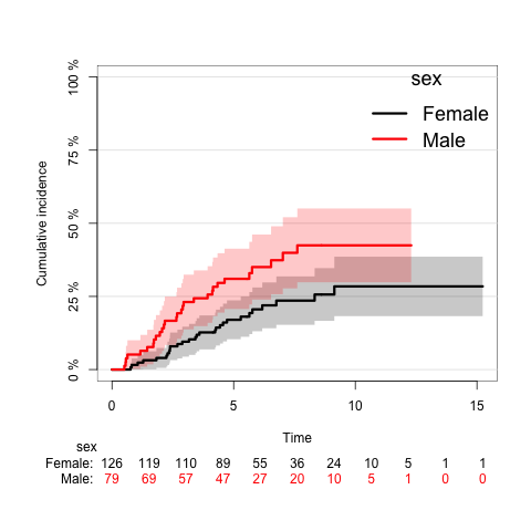
Plot survival curve of competing risk analysis with prodlim (default)
# Default plot
plot(CompRskAnalysis2)
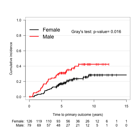
Plot survival curve of competing risk analysis with prodlim (modified)
- adjust legend
- add tick-mark at right censoring times
- rotate labels of y-axis
- add statistical significance from results of cuminc described above
- etc
# Plot with modification
plot(CompRskAnalysis2,
     cause = "death.malignant.melanoma",
     xlim=c(0, 15),
     legend.x="topleft", # position of legend
     legend.cex=1.5, # font size of legend
     marktime = TRUE, # the curves are tick-marked at right censoring times by invoking the function markTime.
     legend.title="",
     atrisk.title="",
     axis2.at=seq(0,1,0.2),
     background.horizontal=seq(0,1,0.2),
     axis2.las=2,                            # rotate labels of y-axis
     percent = FALSE,
     confint = FALSE,
     atrisk.col="black",
     xlab="Time to primary outcome (years)"
     )
text(6.5,0.85,adj=0,paste("Gray's test: p-value=", round(Results_cmprsk$Tests[1,2],3)), cex = 1.2)
今回は,学会発表用のグラフ作成に必要であった.忘れないうちにまとめておく.以前は,at risk tableを別途作成してグラフに合体させるという荒業を行っていたが,これで非常に楽になった.