またまたRネタである.グラフに注釈をつけたくなることがあるが,なかなか見映えのする注釈をつけるのは難しい.最近,それなりの方法を見つけたので,まとめておく.例として,代謝経路の変化を縦型の折れ線グラフで描きKEGG orthologyによって分類したグラフを作成してみる.うーむ,自分で書いていてなんだが,マニアックなネタである...(^^;;;
ま,備忘録として書いておこう.
References
Kyoto Encyclopedia of Genes and Genomes (KEGG) に関しては以下のサイトを参照
Data Preparation
例によって,まず,架空のデータを作成する.Drugを投与して1,5,12,24時間後の代謝物の血中濃度変化を対照,つまり偽薬を投与した群と比較するという実験の結果を適当に作成する.代謝経路はKEGGのデータベースから適当に名前を充てがっておく.
set.seed(100)
data.df1 <- data.frame(
  Pathwayname = c("Cysteine and methionine metabolism","Histidine metabolism","Glucosinolate biosynthesis","Novobiocin biosynthesis","Phenylpropanoid biosynthesis","Pentose phosphate pathway","Cell cycle - yeast","Mineral absorption","Protein digestion and absorption","Type II diabetes mellitus","Insulin secretion","Carbon fixation in photosynthetic organisms","Photosynthesis","Peptidoglycan biosynthesis","Synthesis and degradation of ketone bodies","Cyanoamino acid metabolism","D-Glutamine and D-glutamate metabolism","Taurine and hypotaurine metabolism","GABAergic synapse","Retrograde endocannabinoid signaling","Synaptic vesicle cycle","Pyrimidine metabolism","HIF-1 signaling pathway","Morphine addiction","Nicotine addiction","Aminoacyl-tRNA biosynthesis"),
  C = rnorm(26, mean = 0, sd = 0.1),   # C: control
  OneH = rnorm(26, mean = 2, sd = 2),
  FiveH = rnorm(26, mean = 2, sd = 5),
  TwH = rnorm(26, mean = 4, sd = 10),
  TFH = rnorm(26, mean = 5, sd = 20))

data.df1
levels(data.df1$Pathwayname)
                                   Pathwayname            C       OneH
1           Cysteine and methionine metabolism -0.050219235  0.5595569
2                         Histidine metabolism  0.013153117  2.4618891
3                   Glucosinolate biosynthesis -0.007891709 -0.3154589
4                      Novobiocin biosynthesis  0.088678481  2.4941520
5                 Phenylpropanoid biosynthesis  0.011697127  1.8177729
6                    Pentose phosphate pathway  0.031863009  5.5147512
7                           Cell cycle - yeast -0.058179068  1.7241408
8                           Mineral absorption  0.071453271  1.7776130
9             Protein digestion and absorption -0.082525943  0.6199714
10                   Type II diabetes mellitus -0.035986213  1.5564115
11                           Insulin secretion  0.008988614  2.3658154
12 Carbon fixation in photosynthetic organisms  0.009627446  2.8346466
13                              Photosynthesis -0.020163395  4.1308047
14                  Peptidoglycan biosynthesis  0.073984050  3.9404040
15  Synthesis and degradation of ketone bodies  0.012337950  1.7967415
16                  Cyanoamino acid metabolism -0.002931671  4.8064070
17      D-Glutamine and D-glutamate metabolism -0.038885425 -1.5535513
18          Taurine and hypotaurine metabolism  0.051085626  3.2457348
19                           GABAergic synapse -0.091381419  0.9554333
20        Retrograde endocannabinoid signaling  0.231029682  4.6444619
21                      Synaptic vesicle cycle -0.043808998  1.2731193
22                       Pyrimidine metabolism  0.076406062  4.6381315
23                     HIF-1 signaling pathway  0.026196129  2.0875581
24                          Morphine addiction  0.077340460 -1.7573118
25                          Nicotine addiction -0.081437912  1.1058756
26                 Aminoacyl-tRNA biosynthesis -0.043845057 -1.4771959
        FiveH         TwH         TFH
1   2.8943242  14.0845187 -24.1598745
2  11.4873285 -16.7440475  -3.0061184
3  -9.3596274  12.9682227 -10.5283457
4   6.9023207   3.5000423  -2.3859302
5  -4.9941281  -9.4534931  29.8020292
6  11.1243621 -15.3121153   2.8513238
7   8.9064936  11.0958158   8.4518701
8  -2.1942594   2.4209497  10.0920254
9   0.6900211   6.1636787  -7.2906766
10  1.6557799  12.1736208 -23.5843019
11  0.1055822  21.2717575  -1.6195087
12 14.9097946   2.9622971   7.5677213
13  2.6491707  -1.5712229  25.3623998
14 -1.5651249  18.2830143  -0.1114738
15  5.1899712  -4.9295740  -1.0508202
16  3.0084580  -7.5757124  37.3038137
17  1.6504153  -1.3029645 -10.4742671
18  1.5375506  28.4568276  13.4800480
19  4.2445164  -4.3249580  -6.6789396
20 -3.3217784   8.1351985  13.3007136
21 -3.8120966  -7.7868314 -25.9052331
22 10.2426087  -7.7403476  -5.3749901
23 -8.3104801   0.6707665  -0.5958311
24  2.0637486  17.6311371  25.1491476
25 -3.4376417  -0.6914734  -4.3913991
26  3.3526975  12.4287563  10.9579408

 [1] "Aminoacyl-tRNA biosynthesis"
 [2] "Carbon fixation in photosynthetic organisms"
 [3] "Cell cycle - yeast"
 [4] "Cyanoamino acid metabolism"
 [5] "Cysteine and methionine metabolism"
 [6] "D-Glutamine and D-glutamate metabolism"
 [7] "GABAergic synapse"
 [8] "Glucosinolate biosynthesis"
 [9] "HIF-1 signaling pathway"
[10] "Histidine metabolism"
[11] "Insulin secretion"
[12] "Mineral absorption"
[13] "Morphine addiction"
[14] "Nicotine addiction"
[15] "Novobiocin biosynthesis"
[16] "Pentose phosphate pathway"
[17] "Peptidoglycan biosynthesis"
[18] "Phenylpropanoid biosynthesis"
[19] "Photosynthesis"
[20] "Protein digestion and absorption"
[21] "Pyrimidine metabolism"
[22] "Retrograde endocannabinoid signaling"
[23] "Synaptic vesicle cycle"
[24] "Synthesis and degradation of ketone bodies"
[25] "Taurine and hypotaurine metabolism"
[26] "Type II diabetes mellitus"
Pathwaynameのlevelsを変更する.KEGG orthologyに合わせた配置にするためである.
data.df1$Pathwayname <- factor(data.df1$Pathwayname,
                               levels = c("Aminoacyl-tRNA biosynthesis", "Nicotine addiction", "Morphine addiction", "HIF-1 signaling pathway", "Pyrimidine metabolism", "Synaptic vesicle cycle", "Retrograde endocannabinoid signaling", "GABAergic synapse", "Taurine and hypotaurine metabolism", "D-Glutamine and D-glutamate metabolism", "Cyanoamino acid metabolism", "Synthesis and degradation of ketone bodies", "Peptidoglycan biosynthesis", "Photosynthesis", "Carbon fixation in photosynthetic organisms", "Insulin secretion", "Type II diabetes mellitus", "Protein digestion and absorption", "Mineral absorption", "Cell cycle - yeast", "Pentose phosphate pathway", "Phenylpropanoid biosynthesis", "Novobiocin biosynthesis", "Glucosinolate biosynthesis", "Histidine metabolism", "Cysteine and methionine metabolism"),
                               labels = c("Aminoacyl-tRNA biosynthesis", "Nicotine addiction", "Morphine addiction", "HIF-1 signaling pathway", "Pyrimidine metabolism", "Synaptic vesicle cycle", "Retrograde endocannabinoid signaling", "GABAergic synapse", "Taurine and hypotaurine metabolism", "D-Glutamine and D-glutamate metabolism", "Cyanoamino acid metabolism", "Synthesis and degradation of ketone bodies", "Peptidoglycan biosynthesis", "Photosynthesis", "Carbon fixation in photosynthetic organisms", "Insulin secretion", "Type II diabetes mellitus", "Protein digestion and absorption", "Mineral absorption", "Cell cycle - yeast", "Pentose phosphate pathway", "Phenylpropanoid biosynthesis", "Novobiocin biosynthesis", "Glucosinolate biosynthesis", "Histidine metabolism", "Cysteine and methionine metabolism"))
levels(data.df1$Pathwayname)
 [1] "Aminoacyl-tRNA biosynthesis"
 [2] "Nicotine addiction"
 [3] "Morphine addiction"
 [4] "HIF-1 signaling pathway"
 [5] "Pyrimidine metabolism"
 [6] "Synaptic vesicle cycle"
 [7] "Retrograde endocannabinoid signaling"
 [8] "GABAergic synapse"
 [9] "Taurine and hypotaurine metabolism"
[10] "D-Glutamine and D-glutamate metabolism"
[11] "Cyanoamino acid metabolism"
[12] "Synthesis and degradation of ketone bodies"
[13] "Peptidoglycan biosynthesis"
[14] "Photosynthesis"
[15] "Carbon fixation in photosynthetic organisms"
[16] "Insulin secretion"
[17] "Type II diabetes mellitus"
[18] "Protein digestion and absorption"
[19] "Mineral absorption"
[20] "Cell cycle - yeast"
[21] "Pentose phosphate pathway"
[22] "Phenylpropanoid biosynthesis"
[23] "Novobiocin biosynthesis"
[24] "Glucosinolate biosynthesis"
[25] "Histidine metabolism"
[26] "Cysteine and methionine metabolism"
データの整形を行う.reshapeのmeltでlong formatのデータにする.
library(reshape)
data_melt.df1 <- melt(data.df1)
head(data_melt.df1)
Using Pathwayname as id variables

                         Pathwayname variable        value
1 Cysteine and methionine metabolism        C -0.050219235
2               Histidine metabolism        C  0.013153117
3         Glucosinolate biosynthesis        C -0.007891709
4            Novobiocin biosynthesis        C  0.088678481
5       Phenylpropanoid biosynthesis        C  0.011697127
6          Pentose phosphate pathway        C  0.031863009
これで解析用のデータが出来上がった.
Plot vertical line graph
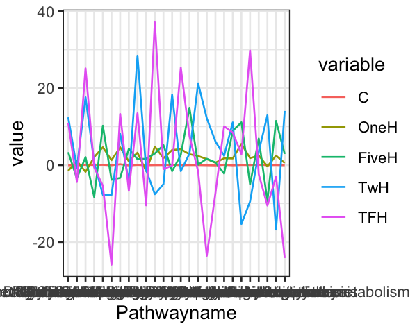
いきなり,Pathwaynameをy軸に設定すると全てのポイントが連結されたグラフになってしまうので,まず,Pathwaynameをx軸に設定して折れ線グラフを描く.
library(ggplot2)
LinePlot_H <- ggplot(data_melt.df1, aes(x = Pathwayname, y = value, group = variable)) +
  theme_bw()
LinePlot_H + geom_line(aes(colour = variable))
Flip the plot so that horizontal becomes vertical with coord_flip
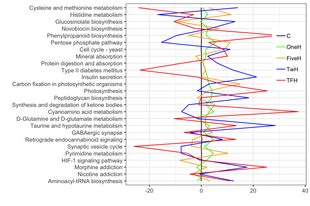
勿論,これではダメなので,coord_flipでx軸とy軸をひっくり返す.また,色もかえる.さらに,x軸とy軸のタイトルを除き,凡例を中に入れて,そのタイトルを除く.
LinePlot_V <- ggplot(data_melt.df1, aes(x = Pathwayname, y = value, group = variable)) +
  theme_bw()
P1 <- LinePlot_V +
  geom_line(aes(colour = variable)) +
  scale_color_manual(values = c("black", "green", "orange", "blue", "red")) +
  xlab("") +
  ylab("") +
  coord_flip()

P1 + theme(legend.position = c(0.9, 0.7)) + theme(legend.title = element_blank())
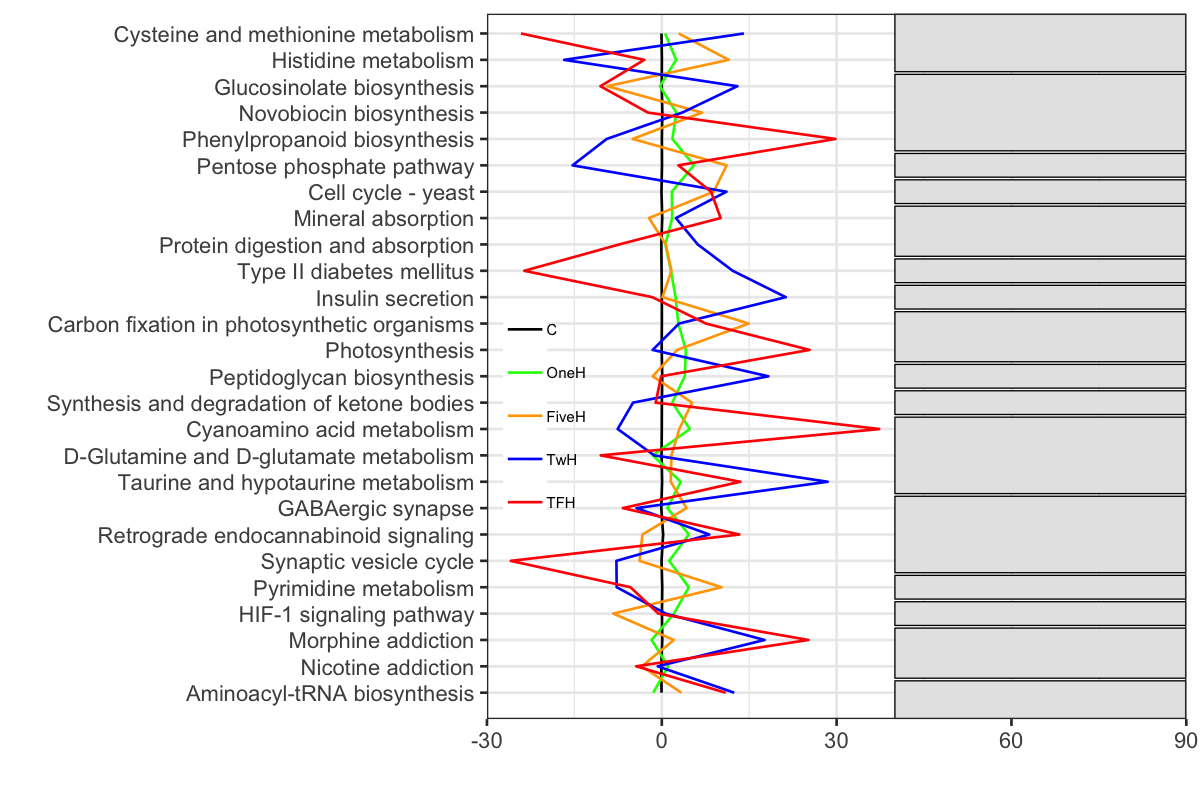
Add annotation box by geom_rect
とりあえずは,それなりの縦向き折れ線グラフが出来上がった.このグラフに注釈ボックスをつけてみる.試行錯誤の結果,ggplot2の場合,geom_rectを使用すれば良いことがわかった.
References
- What is a good way to fit text inside a plotting area with ggplot2 using a pre-defined width for the text?
- ggplot2 Quick Reference: geom_rect
- Adding multiple shadows/rectangles to ggplot2 graph
まず,注釈ボックスとするrectangle用のデータを用意する.
rect1 <- data.frame (xmin=24.55, xmax=26.75, ymin=40, ymax=90, text = data_melt.df1[1,1])
rect2 <- data.frame (xmin=21.55, xmax=24.45, ymin=40, ymax=90, text = data_melt.df1[2,1])
rect3 <- data.frame (xmin=20.55, xmax=21.45, ymin=40, ymax=90, text = data_melt.df1[3,1])
rect4 <- data.frame (xmin=19.55, xmax=20.45, ymin=40, ymax=90, text = data_melt.df1[4,1])
rect5 <- data.frame (xmin=17.55, xmax=19.45, ymin=40, ymax=90, text = data_melt.df1[5,1])
rect6 <- data.frame (xmin=16.55, xmax=17.45, ymin=40, ymax=90, text = data_melt.df1[6,1])
rect7 <- data.frame (xmin=15.55, xmax=16.45, ymin=40, ymax=90, text = data_melt.df1[7,1])
rect8 <- data.frame (xmin=13.55, xmax=15.45, ymin=40, ymax=90, text = data_melt.df1[8,1])
rect9 <- data.frame (xmin=12.55, xmax=13.45, ymin=40, ymax=90, text = data_melt.df1[9,1])
rect10 <- data.frame (xmin=11.55, xmax=12.45, ymin=40, ymax=90, text = data_melt.df1[10,1])
rect11 <- data.frame (xmin=8.55, xmax=11.45, ymin=40, ymax=90, text = data_melt.df1[11,1])
rect12 <- data.frame (xmin=5.55, xmax=8.45, ymin=40, ymax=90, text = data_melt.df1[12,1])
rect13 <- data.frame (xmin=4.55, xmax=5.45, ymin=40, ymax=90, text = data_melt.df1[13,1])
rect14 <- data.frame (xmin=3.55, xmax=4.45, ymin=40, ymax=90, text = data_melt.df1[14,1])
rect15 <- data.frame (xmin=1.55, xmax=3.45, ymin=40, ymax=90, text = data_melt.df1[15,1])
rect16 <- data.frame (xmin=0, xmax=1.45, ymin=40, ymax=90, text = data_melt.df1[16,1])
Remove right margin with expand=c(0,0)
ボックスの右端を90にしたので,グラフがはみ出さないように,scale_y_continuousを用いて,expand=c(0,0)で余白を省き,limitsで軸の範囲を指定する.凡例の位置も変え,背景を透明にして,フォントサイズも小さくする.
P2 <- P1 + theme(legend.position = c(0.0825, 0.43)) +
  theme(legend.title = element_blank(),
        legend.text =  element_text(size = 6),
        legend.background = element_blank())       # legendの背景を透明にする
P2

P3 <- P2 +
  geom_rect(data=rect1, aes(xmin=xmin, xmax=xmax, ymin=ymin, ymax=ymax), fill="grey90", alpha=1, color="black", lwd = 0.25, inherit.aes = FALSE) +
  geom_rect(data=rect2, aes(xmin=xmin, xmax=xmax, ymin=ymin, ymax=ymax), fill="grey90", alpha=1, color="black", lwd = 0.25, inherit.aes = FALSE) +
  geom_rect(data=rect3, aes(xmin=xmin, xmax=xmax, ymin=ymin, ymax=ymax), fill="grey90", alpha=1, color="black", lwd = 0.25, inherit.aes = FALSE) +
  geom_rect(data=rect4, aes(xmin=xmin, xmax=xmax, ymin=ymin, ymax=ymax), fill="grey90", alpha=1, color="black", lwd = 0.25, inherit.aes = FALSE) +
  geom_rect(data=rect5, aes(xmin=xmin, xmax=xmax, ymin=ymin, ymax=ymax), fill="grey90", alpha=1, color="black", lwd = 0.25, inherit.aes = FALSE) +
  geom_rect(data=rect6, aes(xmin=xmin, xmax=xmax, ymin=ymin, ymax=ymax), fill="grey90", alpha=1, color="black", lwd = 0.25, inherit.aes = FALSE) +
  geom_rect(data=rect7, aes(xmin=xmin, xmax=xmax, ymin=ymin, ymax=ymax), fill="grey90", alpha=1, color="black", lwd = 0.25, inherit.aes = FALSE) +
  geom_rect(data=rect8, aes(xmin=xmin, xmax=xmax, ymin=ymin, ymax=ymax), fill="grey90", alpha=1, color="black", lwd = 0.25, inherit.aes = FALSE) +
  geom_rect(data=rect9, aes(xmin=xmin, xmax=xmax, ymin=ymin, ymax=ymax), fill="grey90", alpha=1, color="black", lwd = 0.25, inherit.aes = FALSE) +
  geom_rect(data=rect10, aes(xmin=xmin, xmax=xmax, ymin=ymin, ymax=ymax), fill="grey90", alpha=1, color="black", lwd = 0.25, inherit.aes = FALSE) +
  geom_rect(data=rect11, aes(xmin=xmin, xmax=xmax, ymin=ymin, ymax=ymax), fill="grey90", alpha=1, color="black", lwd = 0.25, inherit.aes = FALSE) +
  geom_rect(data=rect12, aes(xmin=xmin, xmax=xmax, ymin=ymin, ymax=ymax), fill="grey90", alpha=1, color="black", lwd = 0.25, inherit.aes = FALSE) +
  geom_rect(data=rect13, aes(xmin=xmin, xmax=xmax, ymin=ymin, ymax=ymax), fill="grey90", alpha=1, color="black", lwd = 0.25, inherit.aes = FALSE) +
  geom_rect(data=rect14, aes(xmin=xmin, xmax=xmax, ymin=ymin, ymax=ymax), fill="grey90", alpha=1, color="black", lwd = 0.25, inherit.aes = FALSE) +
  geom_rect(data=rect15, aes(xmin=xmin, xmax=xmax, ymin=ymin, ymax=ymax), fill="grey90", alpha=1, color="black", lwd = 0.25, inherit.aes = FALSE) +
  geom_rect(data=rect16, aes(xmin=xmin, xmax=xmax, ymin=ymin, ymax=ymax), fill="grey90", alpha=1, color="black", lwd = 0.25, inherit.aes = FALSE)

P3 + scale_y_continuous(expand=c(0,0), limits = c(-30, 90))
customize tick marks with limits and breaks of scale_y_continuous
ggplot2 axis ticks : A guide to customize tick marks and labels
ticksを指定する.範囲も指定する.scale_y_continuousのlimitsとbreaksは別々に書くとお互いを上書きするので,同じ () の中で書くようにすると両方ともが効くようになる.
R ggplot2 scale_y_continuous : Combining breaks & limits
P4 <- P3 +
  scale_y_continuous(expand=c(0,0), limits = c(-30, 90), breaks=c(-20, 0, 20, 40))
P4
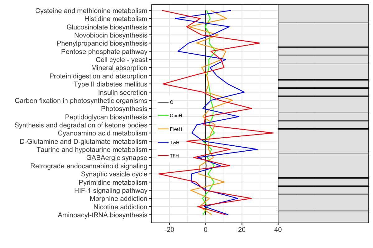
これで空白の注釈用ボックスができた.
Add KEGG orthology (KO)
ggplot2 Quick Reference: geom_rect
上記サイトを参考にして,空白のボックスに該当するKOを記入する.
P4 +
  geom_text(data = rect1, aes(x=xmin+(xmax-xmin)/2, y=ymin+(ymax-ymin)/2, label= "Amino acid metabolism"), inherit.aes = FALSE, size = 2.4) +
  geom_text(data = rect2, aes(x=xmin+(xmax-xmin)/2, y=ymin+(ymax-ymin)/2, label= "Biosynthesis of \n other secondary metabolites"), inherit.aes = FALSE, size = 2.4) +
  geom_text(data = rect3, aes(x=xmin+(xmax-xmin)/2, y=ymin+(ymax-ymin)/2, label= "Carbohydrate metabolism"), inherit.aes = FALSE, size = 2.4) +
  geom_text(data = rect4, aes(x=xmin+(xmax-xmin)/2, y=ymin+(ymax-ymin)/2, label= "Cell growth and death"), inherit.aes = FALSE, size = 2.4) +
  geom_text(data = rect5, aes(x=xmin+(xmax-xmin)/2, y=ymin+(ymax-ymin)/2, label= "Digestive system"), inherit.aes = FALSE, size = 2.4) +
  geom_text(data = rect6, aes(x=xmin+(xmax-xmin)/2, y=ymin+(ymax-ymin)/2, label= "Endocrine and metabolic disease"), inherit.aes = FALSE, size = 2.4) +
  geom_text(data = rect7, aes(x=xmin+(xmax-xmin)/2, y=ymin+(ymax-ymin)/2, label= "Endocrine system"), inherit.aes = FALSE, size = 2.4) +
  geom_text(data = rect8, aes(x=xmin+(xmax-xmin)/2, y=ymin+(ymax-ymin)/2, label= "Energy metabolism"), inherit.aes = FALSE, size = 2.4) +
  geom_text(data = rect9, aes(x=xmin+(xmax-xmin)/2, y=ymin+(ymax-ymin)/2, label= "Glycan biosynthesis and metabolism"), inherit.aes = FALSE, size = 2.4) +
  geom_text(data = rect10, aes(x=xmin+(xmax-xmin)/2, y=ymin+(ymax-ymin)/2, label= "Lipid metabolism"), inherit.aes = FALSE, size = 2.4) +
  geom_text(data = rect11, aes(x=xmin+(xmax-xmin)/2, y=ymin+(ymax-ymin)/2, label= "Metabolism of other amino acids"), inherit.aes = FALSE, size = 2.4) +
  geom_text(data = rect12, aes(x=xmin+(xmax-xmin)/2, y=ymin+(ymax-ymin)/2, label= "Nervous system"), inherit.aes = FALSE, size = 2.4) +
  geom_text(data = rect13, aes(x=xmin+(xmax-xmin)/2, y=ymin+(ymax-ymin)/2, label= "Nucleotide metabolism"), inherit.aes = FALSE, size = 2.4) +
  geom_text(data = rect14, aes(x=xmin+(xmax-xmin)/2, y=ymin+(ymax-ymin)/2, label= "Signal transduction"), inherit.aes = FALSE, size = 2.4) +
  geom_text(data = rect15, aes(x=xmin+(xmax-xmin)/2, y=ymin+(ymax-ymin)/2, label= "Substance dependence"), inherit.aes = FALSE, size = 2.4) +
  geom_text(data = rect16, aes(x=xmin+(xmax-xmin)/2, y=ymin+(ymax-ymin)/2, label= "Translation"), inherit.aes = FALSE, size = 2.4)
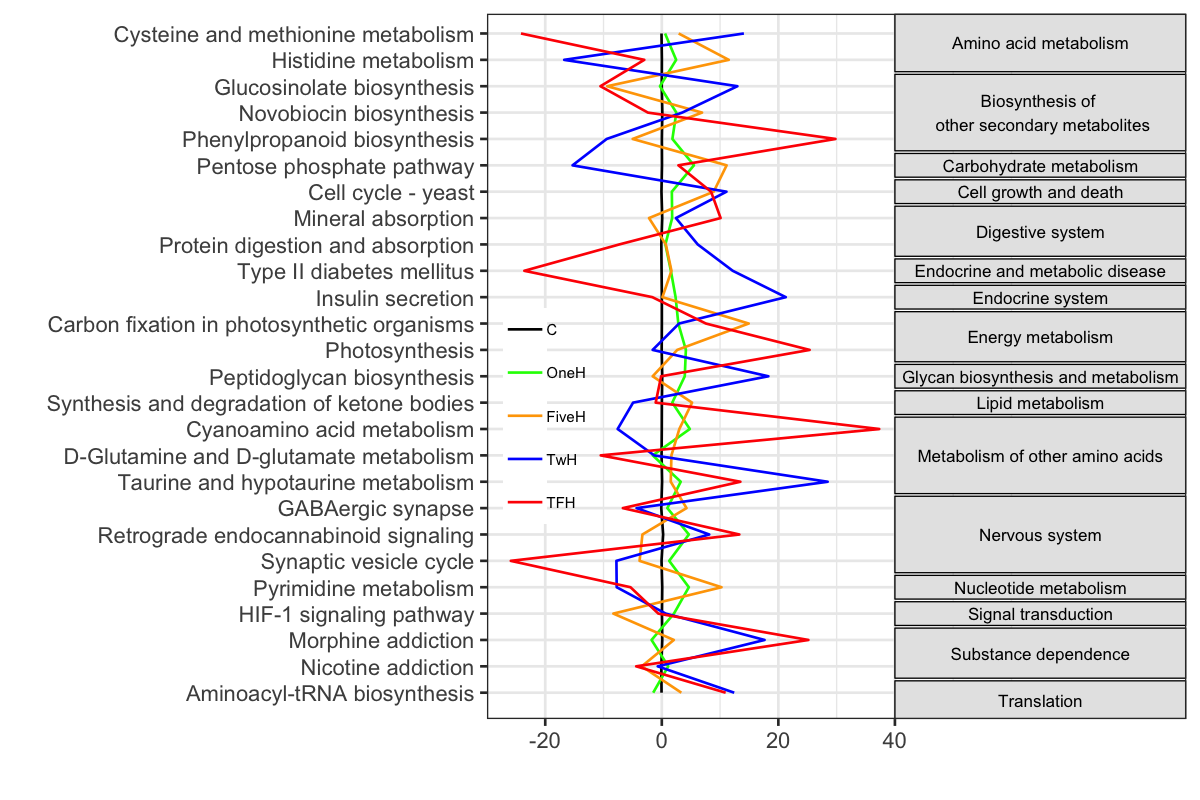
ようやく完成である.この方法は他のタイプのグラフにも使えると思う.もっと簡単な方法があれば良いのだが...